
Volatility may sound like a dirty word in investing, but it’s an everyday fact of life. Even when markets are relatively calm, there is always some level of volatility. That turbulence may burst into the open when an economic crisis strikes, but volatility can be a valuable signal to investors in both good and bad times.
However, while volatility might be easy to identify — like big swings in asset prices — it’s often much harder to quantify. That’s where the volatility index (VIX) comes into play. As an index built to measure future stock market volatility, the VIX is generally considered in the industry as pivotal to informed investment decision-making by supplying traders, asset managers and others with hard data on volatility.
Yet what does a VIX level of 15.4 or 65.8 mean? Stock index values are reflective of stock prices, but how is the VIX calculated?
To help answer the question, we’re going to take a look at the complex calculation behind the VIX.
The VIX in a nutshell
Before diving headfirst into the methodology, let’s back up and first define exactly what the VIX is.
The VIX was first introduced by the Chicago Board Options Exchange (CBOE), now known as Cboe Global Markets (Cboe), in 1993. The index is a financial benchmark meant to measure the market’s expectations for future volatility. It’s often referred to as the “Fear Index” or “Fear Gauge” because, historically, spikes in the VIX have occurred at the same time as financial crises.
According to Cboe, the VIX is “intended to provide an instantaneous measure of how much the market expects the S&P 500 will fluctuate in the 30 days from the time of each tick of the VIX Index.”
Whereas the components of a stock index are equities, the components of the VIX are options. Specifically, they are options contracts for the S&P 500 (SPX) — and the calculation uses real-time bid/ask quotes to compute expected volatility of the SPX.
Robert Whaley, a professor of management at Vanderbilt University, is credited with creating the calculation behind the VIX. Hired by CBOE to build an implied volatility index, Whaley developed the methodology and helped introduce the VIX in ’93, back when it tracked S&P 100 options. The calculation underwent an update in 2003 to use S&P 500 options, which by that time had taken over S&P 100 options in trading volume. Goldman Sachs assisted in the transformation, which also led to the inclusion of out-of-the money puts to better represent the market for options.
And if you were to ask Whaley, the “fear gauge” moniker of the VIX, while good for headlines, isn’t altogether accurate. For him, the VIX represents the price of insurance, or what premium options traders are willing to pay to hedge their risks.
How is the VIX calculated?
Although the formula is complex, there are a few basic points to understand about how the VIX is calculated:
- Implied volatility: Technically, a VIX reading expresses implied volatility, or future expectations. This is in contrast to realized volatility, which can be calculated using historical price data.
- Eligible options: Put and call options selected for the calculation have both weekly and monthly expiration. Put options give the buyer the right to sell, whereas call options give the buyer the right to buy the asset. The eligible range of options have more than 23 days but fewer than 37 days until expiration.
- Range of options prices: Options that are selected can occur across a range of strike prices (or the price level at which option contracts can be exercised). These include both out-of-the-money and at-the-money options.
- Calculated twice: In order to reach the VIX value, the calculation is run twice: once for near-term options and again for next-term options.
Now, let’s walk through a step-by-step calculation of the VIX, drawing heavily on the methodology white paper published by Cboe.
1 | The equation and its variables
The general formula for the VIX is:
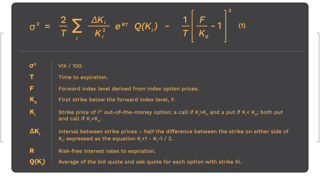
2 | Determine ‘T’ and ‘R’
The process starts with calculating time to expiration and the risk-free interest rate.
For reasons of precision, the calculation measures T in calendar days that are divided into minutes. It works like this:
- N = MCurrent day + MSettlement day + MOther days
- T = N / Minutes in a year
Where:
- MCurrent day equals the minutes remaining until midnight of the current day.
- MSettlement day equals the minutes from midnight until 8:30 a.m. for standard third-Friday AM-settled SPX expirations; or minutes from midnight until 3:00 p.m. for weekly, PM-settled SPX expirations.
- MOther days| equals the total minutes in the days between the current day and settlement day.
For this example, let’s assume that it’s 10:00 in the morning, the near-term options are standard and have 24 days to expire, and the next-term options are weekly and have 31 days to expire.
T1 is (840 + 510 + 33,120) / 525,600 = 0.0655822
T2 is (854 + 900 + 43,200) / 525,600 = 0.0855289
Regarding the risk-free interest rates, R1 and R2, the value of these variables is based on bond-equivalent yield for U.S. Treasury bills that mature closest to the option cycle. Different values may be used for the risk-free rates.
For this purpose of this example, R is 0.11% for the near term and 0.13% for the next term.
3 | Determine ‘F’ and select options
Now onto the real meat of the calculation.
To start, we need to determine where the absolute difference between call and put price quotes is smallest. Let’s assume the following for our near- and next-term options, with strike price being the value the SPX trades at.
| Strike | Call | Put | Difference | Call | Put | Difference |
| 2,995 | 207.10 | 199.60 | 7.50 | 210.60 | 201.10 | 9.5 |
| 3,000 | 204.55 | 203.05 | 1.50 | 208.55 | 203.05 | 5.50 |
| 3,005 | 201.75 | 206.80 | 5.05 | 206.75 | 205.80 | 0.95 |
| 3,010 | 198.60 | 210.45 | 11.85 | 203.60 | 208.45 | 4.85 |
The formula for F is as follows:
F = Strike Price + e(RT) x (Call Price – Put Price)
With these values, we can see the smallest difference for the near-term occurs at 3,000 and 3,005 for the next-term and begin to calculate F for both cycles:
F1 is 3,000 + e(0.0011 x 0.0655822) x (204.55 – 203.05) = 3,001.50011
F2 is 3,005 + e(0.0013 x 0.0855289) x (206.85 – 205.80) = 3,005.95010
Now, let’s address how to select options. The eligible pool of options compromises out-of-the-money SPX calls and puts that center around an at-the-money strike, which is K0. This is the strike price immediately below the forward index level. In this example, the K0,1 is 3,000 and K0,2 is 3,005.
We start collecting options with out-of-the-money puts that have a strike price lower than K0. Beginning immediately below K0, put options are selected, excluding those with a bid equal to zero (i.e., no bid). The process stops once two consecutive puts occur with no bid; that means puts with bids that occur after the two consecutive zero bids are notconsidered.
Those steps are repeated for calls, except we’re moving upward to collect calls with a strike price above K0. The same rules apply — zero bid options are not considered, nor are those with a bid that occur after two consecutive no bids. Finally, both the at-the-money put and call at strike price K0 are selected.
4 | Determine each eligible option’s price and contribution
In this part, we’re talking about these two parts of the general formula:
- Q(K1)
- The summation of ∑1 ΔK1 / K12
These two pieces refer to the calculation of an individual option’s price and contribution to volatility.
Let’s tackle price first. The price of each put with a strike price < K0 and each call with a strike price > K0 is equal to the midpoint of the option’s bid and ask. Whereas K0 is the at-the-money option, Ki refers to the individual option at each strike price collected below or above until two non-bid options occur. Remember, options prices are determined for both the near and next terms.
Q(Ki<K0) = (Put Bidi + Put Aski) / 2
Q(Ki>K0) = (Call Bidi + Call Aski) / 2
It works a bit different for the at-the-money strikes, which are average into a single value.
Q(Ki=K0) = (Put Bidi + Put Aski + Call Bidi + Call Aski) / 4
The summation portion (∑…) is simply the process of determining each option’s contribution to volatility. In general, the further away from the at-the-money strike, the less influence an option will have on either near or next-term volatility. Generally, ΔK1 is half the difference between strikes prices on either side of the option. When at the lower or upper limit, ΔK1 is the difference between Ki and the adjacent strike.
Now, we’re going to try to put these numbers into action. Let’s consider a near-term put at 2,400 with a midpoint bid/ask spread of 0.125. On either side of it are put bids at strikes of 2,390 and 2,420; thus ΔK2400 is 15.
To determine its contribution, we start with ΔK1 / K12 x eRT x Q(Ki), which becomes ΔK2400 Put / K2400 Put2 x eRT x Q(2400 Put). Once all the variables are plugged in, it looks like:
15 / 24002 x e(0.0011 x 0.0655822) x (0.125) = 0.00000033
As seen, the contribution of the 2,400 put to near-term volatility is small because it’s so far out of the money. This calculation is performed for each eligible option.
5 | Calculate near- and next-term volatility
Now we have all we need to calculate volatility for both cycles. It’s an easier equation to tackle if you break down the general formula into two main parts:
- 2 / T x ∑1 ΔK1 / K12 x eRT x Q(K1)
- 1 / T [F / Ko – 1]2
When put together, σ2 for both near and next terms will be calculated. Let’s assume that after summing the value for each eligible option, the contribution by strike is equal to 0.4028499 for the near term and 0.3677285 for the next term, similar to an example in a CBOE white paper from 2009.
Now it’s time to solve that second portion.
For the near term (σ21):
1 / 0.0655822 x [3,001.50011 / 3,000 – 1]2 = 0.0000038
For the next term (σ22):
1 / 0.0855289 x [3,005.95010 / 3,005 – 1]2 = 0.0000012
Put the two together, aaaand:
σ21 is 0.4028499 – 0.0000038 = 0.4028461
σ22 is 0.3677285 – 0.0000012 = 0.3677273
6 | Calculate the 30-day weighted average
Thought we were done? Not quite!
The final step is to plug those near and next-term values into an equation that produces a 30-day weighted average. The square root of that value is multiplied by 100 to get the VIX, which looks like this:
VIX = 100 x √ {T1σ21[NT2 – N30 / NT2 – NT1] + T2σ22[N30 – NT1 / NT2 – NT1]} x N365 / N30
Where:
- NT1 = number of minutes to expiration of the near-term options (34,560 in this case)
- NT2 = number of minutes to expiration of the next-term options (44,640)
- N30 = number of minutes in 30 days (43,200)
- N365 = number of minutes in a 365-day year (525,600)
100 x √ {0.0655822 x 0.4028461[44,640 – 43,200 / 44,640 – 34,560] + 0.0855289 x 0.3677273[43,200 – 34,560 / 44,640 – 34,560]} x 525,600 / 43,200
Using the values of our hypothetical example, we get a final VIX value of 57.60.
How Magma uses the VIX
While we used arbitrary numbers for this example, we believe a VIX reading of 57.60 might indicate the market expects a medium to high level of volatility to occur in the next month. This could lead investors to alter strategies to protect or otherwise grow their portfolios.
Magma Capital Funds depends on the VIX in the investment decision-making process. For example, we allocate the assets of the Magma Total Return Fund if the VIX reaches certain thresholds. Because asset classes have been proven to rise and fall over time, we believe volatility is a key indicator to stages of economic cycles.
Want to learn more about the Magma Total Return Fund or how to invest? Contact us today.